Auckland Meccano Guild
Differential Analyser Explained
Articles
THE DIFFERENTIAL ANALYSER EXPLAINED
by William Irwin
(updated July 2009)
Introduction.
The mechanical Differential Analyser has intrigued mathematically minded Meccanomen for many years, ever since this machine was first modelled, largely in Meccano, by Douglas Hartree and Arthur Porter at Manchester University in 1934. Many full scale non-Meccano Differential Analysers were built in USA, UK and Europe between 1934 and the early 1950s, until they were eventually replaced by faster digital computers. The unique aspect of the Meccano Differential Analyser was that it was accurate enough for the solution of many scientific problems, and much cheaper to build. It is estimated by Garry Tee of Auckland University that about 15 Meccano model Differential Analysers were built for serious work by scientists and researchers around the world.
Very few of the original Meccano model Differential Analysers have survived. In fact I know of only two. The first is part of the original Meccano Differential Analyser no. 1 built by Hartree and Porter at Manchester, which is currently displayed in the Science Museum in London (see fig. 1 below). The second is right here at the Museum of Transport and Technology (MOTAT) in Auckland, New Zealand, and consists of the entire Meccano Differential Analyser no. 2 built by J.B. Bratt at Cambridge University in 1935. This machine was last displayed at MOTAT in the seventies and early eighties. It has recently been restored for display purposes and has been on public display at MOTAT again from April 2009.
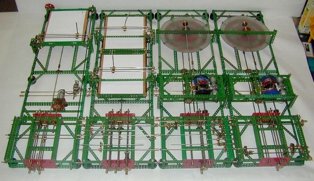
The early Meccano model Differential Analysers were not built entirely of Meccano. The integrator discs were ground glass, and various other parts such as the torque amplifier drums were separately manufactured. Indeed it was considered that a reliable torque amplifier could not be built entirely out of Meccano parts! This has been disproved several times over the years by dedicated Meccanomen. Tim Robinson of California, USA, has perfected the Meccano Differential Analyser to a high accuracy using Meccano parts only, except for the ground glass integrator disc and cord for the torque amplifiers. The picture above is an early example of Tims work, and shows what can be achieved in pure Meccano.
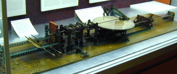
fig. 1
What is a Differential Analyser?
The Differential Analyser is a mechanical analogue computer. What does this mean and where does it fit into the scheme of things?
There are two distinct branches of the computer family. One branch descends from the abacus, which is an extension of finger counting. The devices that stem from the abacus use digits to express numbers, and are called digital computers. These include calculators and electronic digital computers.
The other branch descends from the graphic solution of problems achieved by ancient surveyors. Analogies were assumed between the boundaries of a property and lines drawn on paper by the surveyor. The term analogue is derived from the Greek analogikos meaning by proportion. There have been many analogue devices down the ages, such as the nomogram, planimeter, integraph and slide rule. These devices usually perform one function only. When an analogue device can be programmed in some way to perform different functions at different times, it can be called an analogue computer. The Differential Analyser is such a computer as it can be set up in different configurations, i.e. programmed, to suit a particular problem.
In an analogue computer the process of calculation is replaced by the measurement and manipulation of some continuous physical quantity such as mechanical displacement or voltage, hence such devices are also called continuous computers. The analogue computer is a powerful tool for the modelling and investigation of dynamic systems, i.e. those in which some aspect of the system changes with time. Equations can be set up concerned with the rates of change of problem variables, e.g. velocity versus time. These equations are called Differential Equations, and they constitute the mathematical model of a dynamic system.
The Differential Analyser solves differential equations by integration. It makes use of one or more wheel and disc integrators (or Kelvin-disc integrators), interconnected by shafts in various ways to suit the problem equations. The process of integration can be illustrated by the simple example of the acceleration of a car. This can be represented for input by a curved graph showing speed varying with time. Say one wanted to find out the distance travelled in a certain time, say five minutes. The period of 5 minutes can be divided into much smaller intervals of say 10 seconds each, and assuming a constant speed over each interval from the graph, a distance travelled for each interval is calculated. The sum of the distances travelled in successive intervals is then the total distance travelled. The smaller the interval taken the more accurate will be the result. This is called Integration, and is the function performed by the integrator in a continuous manner.
How does the Differential Analyser Work?
A typical mechanical Differential Analyser consists of the following components:
- Two or more Integrator units (including one Torque Amplifier per unit).
- adding and counting units.
- Input and Output tables.
- A gearing and shafting system to link everything together.
The Integrator:
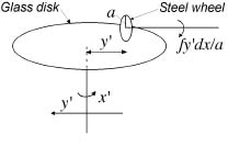
The Integrator is in essence a variable-speed gear, and takes the form of a rotating horizontal disc on which a small knife-edged wheel rests. The principle used is shown in fig. 2. The vertical axis of the horizontal disc is supported in a movable carriage so that the distance of the point of contact of the wheel on the disc, from the centre of the disc, can be varied. The two inputs to the integrator are therefore the rotation of the disc x, and the carriage movement y. When the unit is integrating, the disc rotates and undergoes a translational movement simultaneously. The rotating disc drives the wheel by friction. The rotation of the wheel represents the output of the integrator. For proper operation the wheel must not slip on the disc so the rim of the wheel must be as sharp as possible, usually hardened steel on a polished glass disc.
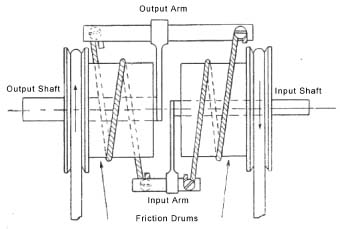
The Torque Amplifier:
The torque on the shaft carrying the integrator wheel is very small due to the low frictional force between the wheel and disc. In order to drive other units of the machine, the shaft from the integrator passes into a Torque Amplifier, the output shaft of which rotates with the same velocity as the input shaft but with greatly increased torque. The principal of the torque amplifier is essentially that of the capstan, where a small force, applied at one end of a friction band wrapped around a rotating drum, produces considerably increased tension at the other end of the band. The principle is shown diagrammatically in fig. 3. The two drums are driven by a motor in opposite directions. Movement of the input shaft tightens the thread on the motor driven drum, which causes the output shaft to rotate with amplified torque. The construction of a Meccano demonstration model of a torque amplifier is described by Michael Adler in the International Meccanoman, no. 34, September 2001.
Adding and Counting Units:
These can be included in the shafting when required. Adding units consist of a differential gear system so arranged that the angular rotation of one shaft connected to it is the sum of the angular rotation of two other shafts. Counters are used when it is desired to know the number of revolutions made by a particular shaft.
Input and Output Tables:
The Input Table is a unit whereby information concerning the differential equation is transmitted to the machine. A stylus is manually made to follow a pre-plotted curve, representing the known functional relationship between the variables. The result is mechanically linked to the input drives. Not all problems require the use of the input table.
The Output Table is similar in construction to the input table. The solution to the equation is drawn by a pen on paper, in the form of a curve, thus plotting the results from the various mechanical linkages.
Operation:
Motors are required for each torque amplifier, and one motor is required for the main input drive. Secondary inputs are manual via the input table. Tim Robinsons fine model above gives the reader a general idea of a typical set-up.
I have purposely not gone into any mathematical background here. Suffice it to say that the Integrators, Input and Output tables, Adders and Counters if required, are all linked together by gearing and shafting to suit the particular differential equation solution required. This requires a lot of effort in setting up for each different problem and is in effect the programming of the machine which defines it as a computer. Of course a thorough knowledge of the mathematics of the problem is required by the user.
Examples of usage:
A practical example of the type of calculation for which the Differential Analyser has been used to predict results is the use by river control authorities in New Zealand for the calculation of soil erosion characteristics of various surface areas. The rate of erosion is among other things dependent upon the following:
1) the rate at which the water is falling on the surfaces
2) the resistance the surface cover offers to the flow of surface water
3) the speed of flow of surface water
4) the volume of water flowing
The Differential Analyser was used in many other fields of science and engineering before being displaced by faster digital computers.
It is rumoured that a differential analyser was used in the development of the "bouncing bomb" by Barnes Wallis for the "Dam Busters" attack on the Ruhr valley hydroelectric dams in WW2. This was first mentioned in MOTAT literature in 1973. However after extensive enquiries and literature searches over the last few years, no evidence can be found that the Differential Analyser no. 2, nor any other differential analyser, was used for this purpose. Considering the secrecy surrounding war time activities at the time it could still be possible, but most people from that era are now deceased. Two remaining personalities still alive from that era were consulted, namely Arthur Porter and Maurice Wilkes, but neither could substantiate the rumour.
References:
Analog Computation, by Albert S Jackson, McGraw Hill 1960
The Differential Analyser, by J Crank, Longmans Green & Co. 1947
Differential Analyser, GMM leaflet no. 4, The Meccanoman's Club, 1967
Torque Amplifiers, by Alan partridge, Constructor Quarterly no. 19, March 1993
Meccano Torque Amplifier, by Michael Adler, International Meccanoman no. 34, September 2001
The Meccano Set Computers, by Tim Robinson, IEEE Control Systems Magazine vol. 25 no. 3, June 2005
re-published in Constructor Quarterly no. 72, June 2006
Acknowledgments:
Lead photograph courtesy of Tim Robinson.
Fig. 1: photograph courtesy of Michael Adler
Other diagrams are by William Irwin.
APPENDIX
For those of a mathematical inclination, the simplest differential equation which can be solved by the Differential Analyser is d2y/dx2 = -y
Since the equation has constant coefficients no manual controls via the input table are required. The output table records dy/dx as a function of y so the plotted output should be a circle. This is known as the "circle test" for accuracy. If there is slippage or any backlash the machine will draw a close spiral instead of a circle.
For other Differential equations the output might be a sine wave (damped or undamped), a plotted trajectory or other curve, depending on the problem being investigated.
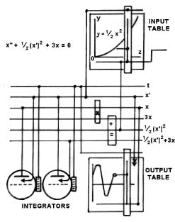
Fig 4 illustrates the differential analyser in diagrammatic form set up to solve a more complicated differential equation involving the use of 2 integrators, input of a function on the input table, and resultant solution in the form of a curve on the output table.